
Variance Tax: The Tax Nobody Told You About
By Dan Snover, CFA, Chief Investment Officer at PMV Capital

About the Author
Dan Snover is the President and Chief Investment Officer at PMV Capital in Dallas, Texas, where he leads the firm’s investment strategy and portfolio construction.
With over 10 years of investment and portfolio construction experience, he has been quoted in the Wall Street Journal and Bloomberg. He was formerly Co-CIO of Fund Architects, LLC, which was acquired by Cabana in 2019, where he led product development, marketing, and distribution of ETF strategies.
A CFA charterholder, Dan is a graduate of the University of Texas at Austin, where he earned a BBA in Accounting from the McCombs School of Business and a BA in Economics with a concentration in macroeconomics.
Your portfolio has two returns: the average return and the compounded return. The return that matters is the one you compound, not the one you average, and volatility is a direct tax on that compounded return.
Take a piece of paper and fold it in half. Then fold it in half again. Keep folding, and after forty-two folds, the stack would reach the moon. A sheet of paper is about 0.1 millimeters thick, so forty-two of them stacked together is less than a quarter of an inch tall. Yet folded, or compounded, the height of the stack reaches roughly 440,000 kilometers into space. This example not only shows the power of compounding, it illustrates the fact that we humans have a difficult time thinking exponentially.
This applies to investing as well. Over time, a large majority of one’s gains are likely the result of compounded returns, while a smaller portion comes from the rate of return itself.
What is not intuitive is that there is a hidden tax, the variance tax (also called the volatility tax), that eats away at your compounded growth rate over time. Reducing this tax is a far more reliable way of improving your performance than trying to beat the market.
Suppose two fund managers are each expected to deliver 10 percent per year for twenty years. At the end of twenty years, one of their clients has nearly double the wealth of the other. The only thing separating the two is how much their returns moved up and down along the way.
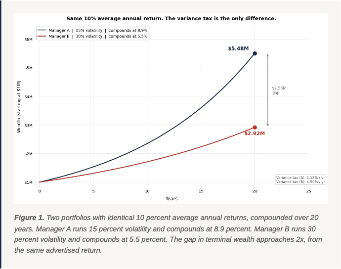
How can that be?
The Compounding Growth Equation
Think about the compounding growth equation that sits underneath every retirement calculator, every financial plan, and every conversation about long-run investing:

The equation says that your future value equals your present value, compounded at a rate of return r over t periods. It is an elegant equation, but it is built on the assumption that returns are constant through time.
In the real world your return is not the same every single period. Returns are a sequence of gains and losses that average out to a single growth rate, so there is a difference between your average return and your compounded return. The gap between the average and the compound return is the variance tax. It is a very real drag, quietly and invisibly deducted from your wealth, that increases with the risk of your portfolio and accumulates over time.
Average Return Versus Compound Return
The fact that every investment, and portfolio of investments, has an average return and a compounded return is not obvious. To illustrate, start with a simple example.
If you gain 10 percent, then lose 10 percent, your average return is zero (+10 − 10 = 0). Yet the compounded growth is not zero.
If you start with $100 and gain 10 percent, the portfolio ends with $110 ($100 × 1.1 = $110). A subsequent 10 percent loss on $110 leaves you with $99 ($110 × 0.9 = $99). The investor has therefore lost one percent despite an average return of zero. The reason is that risk, or volatility, is a tax that eats at your returns over time.
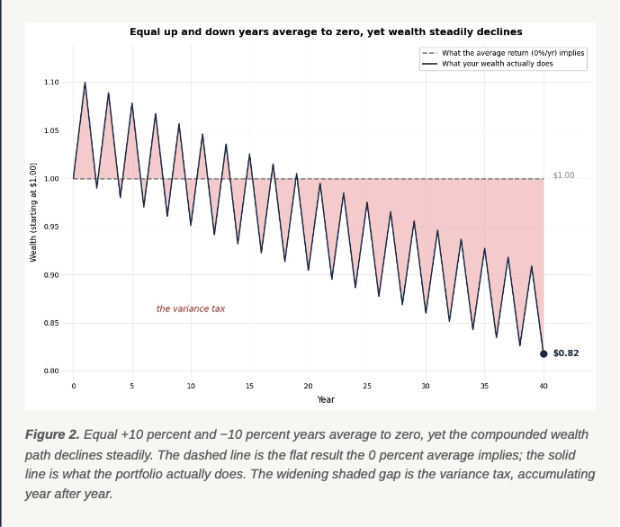
The general rule: for any investment whose returns vary at all, the compounded return is always lower than the arithmetic average. The more the returns vary, the bigger the gap. And that gap is not noise or bad luck. It is a mathematical tax, a structural drain on the wealth you are trying to build.
The Tax Has a Formula
You can estimate the gap caused by the variance tax from a single equation that connects average return, volatility, and the return you actually compound:

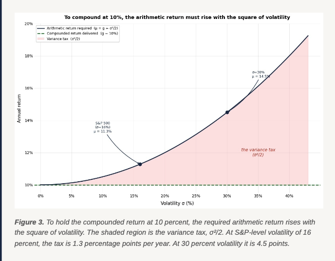
The equation says your compounded growth rate (r) is approximately your average return (μ), minus a penalty equal to half the square of your volatility (σ). The average return (μ) is the engine pulling you forward. The variance tax (−σ²/2) is a drag that grows with the square of how much your returns move around.
That square term in the variance tax is important, because it indicates that a change in risk has an outsized effect on the compounded return. Double your volatility and you quadruple the tax. Halve your volatility and you reduce the tax by three quarters. The tax is not linear. It accelerates, which is why rough return paths destroy wealth so much faster than their averages suggest.
Note that the compounded growth rate (r) calculated from this formula is the rate of return (r) you should use in the original growth equation, FV = PV × (1 + r)^t. The table below shows the size of the tax across a range of volatility levels. Each row holds the compounded return fixed at 10 percent and asks what average return is required to deliver it at each level of volatility:
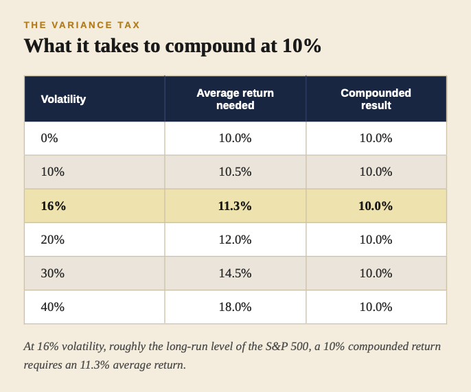
At 16 percent volatility, roughly the long-run level of the S&P 500, a 10 percent compounded return requires an 11.3 percent average return. The tax is invisible in your quarterly statement, but it shows up without fail in the wealth you accumulate over decades.
Why Does the Variance Tax Exist?
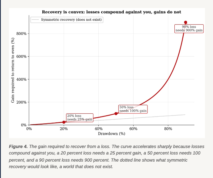
The variance tax exists because a loss requires a proportionally larger gain to undo. This relationship becomes more clear when you look at more extreme losses:
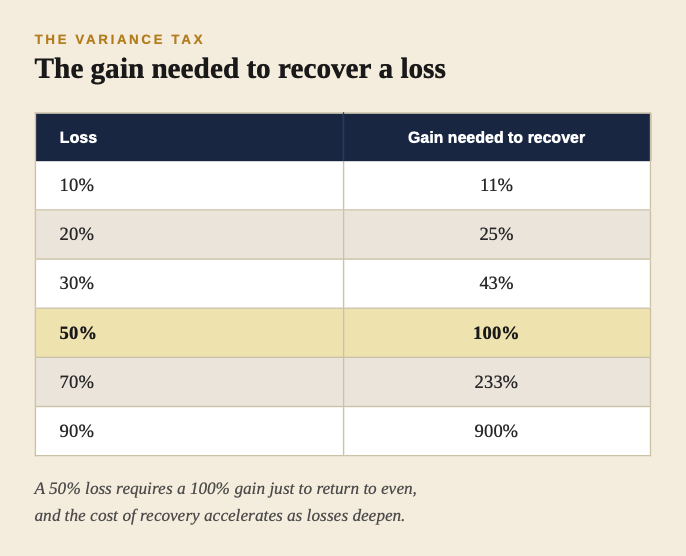
A 50 percent loss requires a 100 percent gain just to return to even. A 90 percent loss requires a ninefold gain. Therefore, every percentage point of volatility you reduce is not just a statistical improvement. It is a real reduction in the compounding drag that operates regardless of the order in which the gains and losses arrive.
Why Volatility Is the Correct Risk Measure
Volatility, which is the up and down swings around your average return, is the risk metric that matters most, because it is the only one that directly impacts the return you keep.
The finance industry uses many different measures of risk, and the list grows longer with every decade of academic research. Maximum drawdown records the peak-to-trough decline. Value at Risk estimates the loss that will be exceeded with some probability over some horizon. Expected Shortfall averages the losses beyond that threshold. Beta measures sensitivity to the market. And on and on. Each of these has a place, but none of them displaces volatility as the measure that belongs in the variance tax formula. There are three reasons for this.
The first is that every other common risk measure is derived from volatility. Value at Risk at 95 percent confidence is approximately 1.65 times the standard deviation. Value at Risk at 99 percent is approximately 2.33 times the standard deviation. Expected Shortfall at 95 percent is approximately 2.06 times the standard deviation. For normally distributed returns these relationships hold exactly, as consequences of the shape of the distribution rather than coincidences. Knowing the volatility of a normally distributed return series tells you the entire loss distribution, and all the other numbers follow.
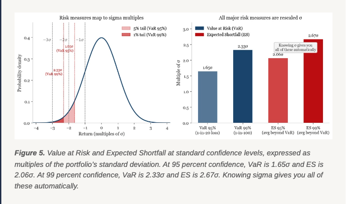
The second reason is that volatility is the quantity that enters the compounding formula. The variance tax is σ²/2. Not the VaR, not the maximum drawdown, not the beta.
The third reason is practical. Volatility is the measure over which investors have the most direct control. You can reduce a portfolio’s volatility through diversification, through the choice of assets, and through the rebalancing rules that govern how the portfolio is maintained. You cannot as directly control the tail of the distribution or the size of the worst drawdown.
Volatility is both the right measure and the actionable one.
None of this denies that fat tails exist, that real return distributions are not perfectly normal, or that the worst outcomes matter disproportionately to investor psychology. But the framework in these articles is not built on the assumption of perfect normality. It is built on the formula r ≈ μ − σ²/2, which holds as an approximation across a wide range of distributions.
What This Article Is Not
The variance tax is the dominant drag on compounded wealth for most long-horizon investors, but it is not the only consideration.
An investor with a fixed liability in the near term, a pension payment due in two years, a house purchase in three, may rightly optimize for something other than maximizing compounded growth. Their horizon is short and their obligation is specific. The framework here is built for the long-horizon wealth-builder, accumulating and eventually spending over decades.
The formula r ≈ μ − σ²/2 is also an approximation. It is exact in continuous time with normally distributed returns and becomes less precise when return distributions have fat tails or structural breaks. The direction and the intuition remain valid across a wide range of real-world conditions, and the mathematical supplement develops the full derivation for readers who want the exact version.
And the indictment of volatility does not mean volatility itself is evil. Risk and return are linked. An investor who eliminates all volatility earns only the risk-free rate. The goal is not to minimize volatility but to minimize it relative to the return it accompanies, which is to say to maximize the ratio of the force to the friction. That ratio has a name, and it is the subject of a future article.
Where This Leads
Your portfolio statement shows one number. That number already has a tax taken out, a variance tax. The riskier the path that produced it, the larger the tax that was deducted before you saw the result. There is no line item for the tax, and it does not appear in any quarterly report. It shows only in the gap between what the portfolio earned on paper and what you actually accumulated over years.
Most investors never see that line, so they never ask the right question: what return am I actually generating, versus what am I losing to the drag of fluctuation? Until you separate those two, you are optimizing for the gross figure and ignoring the deduction.
Every investor paying attention to the right number, the compounded return rather than the average return, now has a precise enemy: the variance tax, equal to half the square of volatility, subtracted from compounded growth every year. It is structural, it is calculable, and it is reducible.
The variance tax is also not spread evenly across a lifetime. The next article shows when it hits hardest. It is survivable while you are saving into a portfolio and punishing once you are spending from one, falling heaviest exactly when you can least afford it.
Compounding is the objective. The variance tax is what stands between you and it.
Today’s article is brought to you by Texas Precious Metals